The consequences of consideration in auditory–visible integration revealed by time-varying networks

People are always uncovered to a plethora of sensory data that they unconsciously combine so as to comprehend their surroundings. Visible and auditory data constitutes the bulk (over 90%) of the knowledge that’s perceived (Treichler, 1967; Ristic and Capozzi, 2023). Auditory–visible integration happens when auditory and visible stimuli coincide temporally and spatially, and when two stimuli are introduced inside an in depth time interval and related spatial association (Stein and Meredith, 1990; Frassinetti et al., 2002; Stevenson et al., 2012; Spence, 2013; Tang et al., 2016; Ľuboš et al., 2021). Consideration performs an important position in selectively processing exterior data and enhancing data processing efficiency by specializing in goal places (Posner and Rothbart, 2006; Zhang T. et al., 2022). Consideration is instrumental in processing dynamic stimuli effectively and enhancing notion, because it directs restricted cognitive assets towards data related to the present job (Tian et al., 2014; Li et al., 2015). As well as, the researches on the eye mechanism might assist to enhance deep neural networks for visible processing duties (Zhang et al., 2019; Wang et al., 2020).

There’s ongoing debate concerning the position of consideration in multisensory integration, notably within the case of auditory–visible integration. Three mainstream theories concerning the relationship between auditory–visible integration and a spotlight have been proposed in earlier research (Koelewijn et al., 2010; Xu et al., 2020). The primary, the early integration framework, asserts that integration happens previous to consideration and might even drive it (Vroomen et al., 2001; Rachel et al., 2022). Proof for that is seen within the “pip-pop impact,” the place the addition of auditory stimulation to a visible search job led to quicker outcomes (Erik et al., 2008). Then non-spatial auditory stimulation was added to the spatial visible experiment. The second principle, the late integration framework, demonstrates that multisensory integration seems behind consideration. In different phrases, two unimodal (i.e., auditory and visible) occasions are attended to individually earlier than they’re built-in. This mannequin signifies that spotlight is important for multisensory integration (Laura et al., 2005; Sébastien et al., 2022). A later examine used a cross-modal consideration desire job to show that cross-modal interactions are influenced by consideration (Romei et al., 2013; Wen et al., 2021). Moreover, late integration means that late cross-modal results are mediated by attentional mechanisms. The third principle is the parallel integration framework; right here, the stage at which multisensory integration takes place is unsure. Multisensory integration may be early or late, and it depends upon experimental or exterior circumstances (Calvert and Thesen, 2004; Sébastien et al., 2022). Some research prolonged the seminal strategies of the parallel integration framework (Talsma et al., 2010; Stoep et al., 2015). This may increasingly produce totally different outcomes on account of a number of components, together with job sort (detection or identification), stimulus properties (easy or complicated), and a spotlight assets (exogenous or endogenous).

Within the examine of the connection between consideration and auditory–visible integration, numerous strategies have been employed. Early analysis utilized behavioral information and found that an auditory stimulus influences the response time (RT) of a synchronous or almost synchronous visible stimulus (Mcdonald et al., 2000; Shams et al., 2000; Laura et al., 2005; Zhang X. et al., 2022) and the reverse can be true (Platt and Warren, 1972; Bertelson, 1999). These outcomes point out {that a} simultaneous or near-simultaneous bimodal stimulus reduces stimulation uncertainty (Calvert et al., 2000), probably supporting the early integration framework or enhancing stimulation response for the late framework (Stein et al., 1989; Zhang et al., 2021). Nonetheless, exterior components, such because the state of the experimental topics, could also be missed.

With the development of mind imaging know-how, growing numbers of researchers have turned to mind imaging to research the connection between consideration and auditory–visible integration. By using an event-related potential part (ERP) of an auditory–visible streaming design and a fast serial visible presentation paradigm, they explored the interactions between multisensory integration and a spotlight (Durk and Woldorff, 2005; Kang-jia and Xu, 2022). The outcomes indicated that exercise related to multisensory integration processes is heightened when they’re attended to, suggesting that spotlight performs a important position in auditory–visible integration and aligning with the late integration standards. The advance of the spatial decision of scalp EEG has lengthy been a topic of curiosity for researchers.

Research utilizing purposeful magnetic resonance imaging (fMRI) with excessive spatial decision have reported the correct location of many areas concerned in auditory–visible integration and a spotlight; these primarily embody the prefrontal, parietal, and temporal cortices (Calvert et al., 2001; Macaluso et al., 2004; Tedersälejärvi et al., 2005; Noesselt et al., 2007; Cappe et al., 2010; Chen et al., 2015).The superior temporal gyrus (STG) and sulcus (STS) each take part in speech auditory–visible integration (Klemen and Chambers, 2012; Rupp et al., 2022) and non-speech auditory–visible stimuli (Yan et al., 2015). Up to now, STG was thought-about an space of pure sound enter (Mesgarani et al., 2014). The temporoparietal junction (TPJ), which is near the STG, is a vital space of the ventral consideration community (VAN) that’s positioned principally in the proper hemisphere, and is recruited in the intervening time a behaviorally related stimulus is detected (Corbetta et al., 2008; Tian et al., 2014; Branden et al., 2022). The TPJ is activated throughout detection of salient stimuli in a sensory surroundings for a visible (Corbetta et al., 2002, 2008), auditory (Alho et al., 2015), and auditory–visible job (Mastroberardino et al., 2015). Nonetheless, as many research have talked about, it’s troublesome to find out precisely the timing traits when utilizing fMRI with poor temporal decision.

Given that EEG and fMRI are two outstanding noninvasive purposeful neuroimaging modalities, they usually exhibit extremely complementary attributes, there was a substantial drive towards integrating these modalities in a multimodal method (Abreu et al., 2018). The mix of scalp EEG’s distinctive temporal decision and fMRI’s exceptional spatial decision permits a extra complete exploration of mind exercise, surpassing the constraints inherent to particular person methods (Bullock et al., 2021). Earlier investigations have examined the purposeful points of the mind in numerous pathological circumstances, equivalent to schizophrenia (Baenninger et al., 2016; Ford et al., 2016). A number of researchers have employed mixture of EEG and fMRI to discover cognitive mechanisms (Jorge et al., 2014; Shams et al., 2015; Wang et al., 2018). Another research have investigated mind dynamics in relation to complicated cognitive processes like decision-making and the onset of sleep (Bagshaw et al., 2017; Pisauro et al., 2017; Hsiao et al., 2018; Muraskin et al., 2018). On this examine, we used these two neuroimaging applied sciences to research the looks order of auditory–visible integration and a spotlight. Earlier research have tended to use a selected experimental paradigm to research this relationship, however few have used community analyses to resolve this conundrum. We employed time-varying community evaluation primarily based on the adaptive directed switch operate (ADTF) methodology to uncover dynamic data processing. This methodology can uncover the dynamic data processing with a multivariate adaptive autoregressive mode (Li et al., 2016; Tian et al., 2018b; Nazir et al., 2020). This method might supply new insights into the temporal order of multisensory integration and a spotlight in a stimulated EEG community.

All through the experiment, a white fixation cross of dimensions (
$0.5°\times 0.5°$
) was introduced on the heart of a black monitor. The visible stimuli consisted of rectangular bins that randomly appeared in both the left or proper visible discipline (LVF or RVF, respectively). The field was $2°\times 2°$ and its width was $0.2°$
. The bins remained on the display for 50 ms and have been adopted by an auditory stimulus, a 1,000 Hz pure tone that additionally randomly appeared within the left or proper auditory discipline (LAF and RAF, respectively) after a 50 or 750 ms interval. Individuals have been instructed to reply by urgent the ‘Z’ key with their left hand if the tone appeared within the LAF, and the ‘/’ key with their proper hand if it appeared within the RAF. Individuals have been required to react as quickly as they heard the pure tone, which lasted for 200 ms. The fixation cross remained on the monitor for an extra 800 ms to make sure individuals had adequate time to reply appropriately. The experimental process is illustrated in Determine 1.

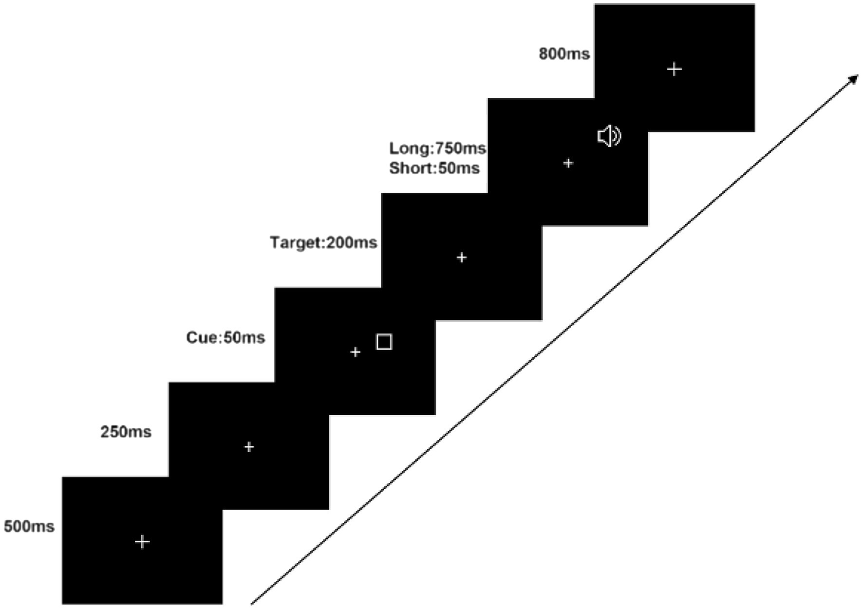
Determine 1. Illustration of stimulus sequence within the experiment.

2.3. Behavioral information and evaluation

The behavioral information was obtained by way of EEG and fMRI. We analyzed RT utilizing repeated measures evaluation of variance (ANOVA) with the next components: stimulus visible discipline (LVF vs. RVF), cue validity (legitimate vs. invalid), stimulus-onset asynchrony (SOA), and the interval between the cue and goal stimulus (lengthy vs. quick). Information consistency was ensured by excluding RTs larger than 900 ms and fewer than 200 ms, in addition to any cases of missed or incorrect key presses.

2.4. EEG and fMRI information recording

Within the examine, EEG and fMRI information have been collected individually. We used a Geodesic Sensor Internet (GSN) with 129-scalp electrodes positioned in response to the Worldwide 10–20 system (Tucker, 1993) to report the EEG at a price of 250 Hz. The Oz, Pz, CPz, Cz, FCz, and Fz electrodes have been positioned in the midst of the cranium, and the remaining electrodes have been distributed alongside either side of the midline. The central prime electrode (Cz) was used because the reference electrode and all electrodes had impedances decrease than 40 kΩ (Tucker, 1993).

fMRI information was collected utilizing the quick T2*-weighted gradient echo EPI sequence on a 3-T GE MRI scanner (TR = 2000 ms, TE = 30 ms, FOV = 24 cm × 24 cm, flip angle = 90°, matrix = 64 × 64, 30 slices) on the College of Digital Science and Know-how of China. This methodology obtained 198 volumes for every session. As a result of the machine at was unstable at the start of the information assortment, we discarded the primary 5 picture volumes of every run for preprocessing.

2.5. The processing framework for time-varying networks

The processing framework for calculating time-varying networks consisted of three phases, as illustrated in Determine 2.

1. ROI choice primarily based on task-related fMRI activations, as proven in Determine 2A.

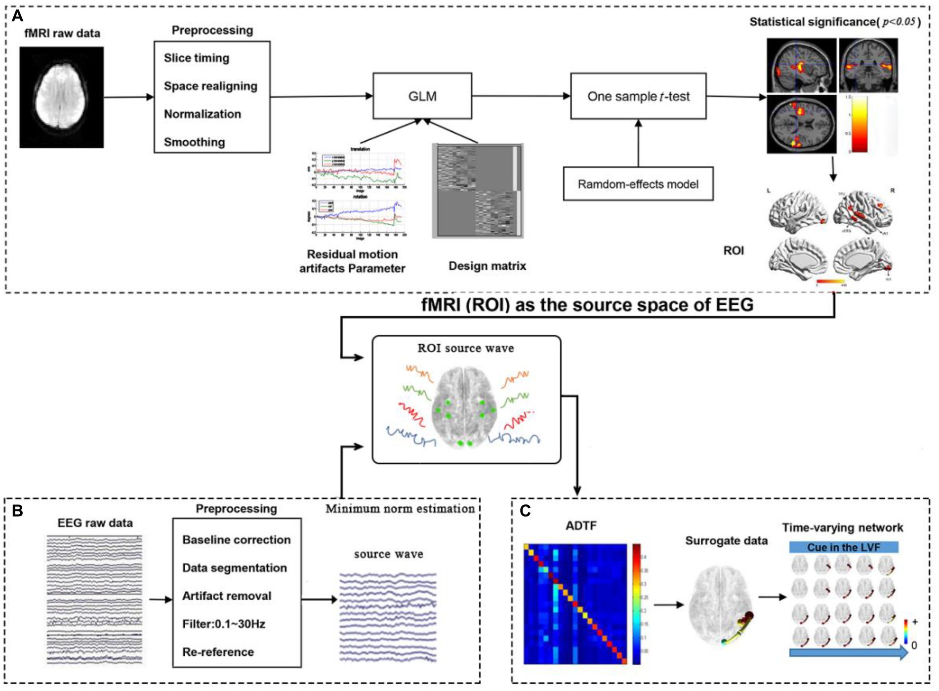
Determine 2. The processing framework for calculating time-varying networks. (A) fMRI processing; (B) EEG processing; (C) Time-varying community developing.

The fMRI information was preprocessed and constructed by a generalized linear mannequin (GLM). The outcomes of the GLM have been then subjected to a statistical check. Reply on the statistical outcomes, 4 activations for the left cue and 4 activations for the proper cue within the fMRI experiment have been chosen as ROIs (nodes) within the cerebral cortex, offering comparatively correct MNI coordinates for the development of the time-varying community within the following steps.

2. Supply wave extraction (Determine 2B).

The EEG information was preprocessed, and the scalp electrical alerts are mapped to the cerebral cortex by MNE supply localization methodology. Then, the MNI coordinates offered by fMRI have been transformed to the corresponding positions of the top mannequin and the corresponding time collection of the cortical electrical alerts are extracted.

3. Time-varying community development (Determine 2C).

Within the third stage, the time-varying community was constructed utilizing the ADTF know-how, primarily based on the outcomes from steps 1 and a couple of.

2.6. fMRI information processing

The remaining volumes underwent preprocessing utilizing Statistical Parametric Mapping model 8 (SPM8) software program. 4 preprocessing pipelines have been utilized on this examine. Firstly, slice timing correction was applied to deal with temporal variations among the many slices. Secondly, spatial realignment was carried out to eradicate head motion, whereby all volumes have been aligned with the primary quantity. Individuals whose head motion exceeded 2 mm or 2 levels have been excluded (Bonte et al., 2014). Thirdly, normalization was carried out to standardize every participant’s unique fMRI picture to the usual Montreal Neurological Institute (MNI) area utilizing EPI templates. Voxel resampling to three × 3 × 3 mm³ was carried out to beat head measurement inconsistencies. Lastly, spatial smoothing was applied to make sure excessive signal-to-noise ratio (SNR) by smoothing the purposeful photos with a Gaussian kernel of full width half most (FWHM) of 6 × 6 × 6 mm³.

After information preprocessing, the time collection of all voxels underwent a high-pass filter at 1/128 Hz and have been then analyzed with a common linear mannequin (GLM; Friston et al., 1995) utilizing SPM8 software program. Temporal autocorrelation was modeled utilizing a first-order autoregressive course of. On the particular person degree, a a number of regression design matrix was constructed utilizing the GLM, that included two experimental occasions primarily based on the cue location (left visible discipline or proper visible discipline). The 2 occasions have been time-locked to the goal of every trial by a canonical artificial hemodynamic response operate (HRF) and its temporal and dispersion derivatives. By together with dispersion derivatives, the evaluation accounted for variations within the period of neural processes induced by the cue location. Nuisance covariates, equivalent to realignment parameters, have been included to account for residual movement artifacts. Parameter estimates have been obtained for every voxel utilizing weighted least-squares, which offered most chance estimators primarily based on the temporal autocorrelation of the information (Wang et al., 2013).

On this examine, to compute easy most important results for every participant, baseline contrasts have been utilized to the experimental circumstances. Subsequently, the ensuing particular person distinction photos have been entered right into a second-level one pattern t-test utilizing a random-effects mannequin. As a way to determine areas of great activation, a threshold of p < 0.05 (false discovery price [FDR] corrected) and a minimal cluster measurement of 10 voxels have been utilized. These stringent standards have been employed to make sure strong and dependable identification of neural activation patterns.

2.7. EEG information preprocessing

The EEG information underwent 5 preprocessing steps. Firstly, the EEG epochs have been set to a time vary of −200 to 1,000 ms. Secondly, we used the common of 200 ms pre-stimulus information as a baseline to appropriate the epochs. Thirdly, we carried out artifact rejection, excluding epochs contaminated by eye blinks, eye actions, amplifier clipping or muscle potentials that exceeded ±75 μv. Fourthly, we filtered the EEG recordings utilizing a band-pass filter of 0.1-30 Hz. Lastly, we re-referenced the information utilizing the reference electrode standardization approach (REST) (Yao et al., 2005; Tian and Yao, 2013; Tian et al., 2018a). We excluded trials with incorrect behavioral responses and dangerous channel replacements, and averaged the ERPs from the stimulus onset time level primarily based on the validity of the cue, visible discipline, and SOA size.

2.8. Minimal norm estimation

The amount conductor impact might result in the era of pseudo-connections throughout mind community development utilizing scalp mind electrical energy. And invasive strategies for instantly amassing mind electrical energy within the cerebral cortex are difficult to make use of. To beat this drawback, we employed supply localization know-how to switch scalp mind electrical sign to the cortex, enabling estimation of cortical electrical alerts (Tian et al., 2018a; Tian and Ma, 2020), and we transformed 129 scalp electrodes into 19 electrodes protecting the entire mind.

On this examine, we used the normalized minimal norm estimation (MNE) supply localization methodology to estimate {the electrical} exercise of the auditory–visible cortex. In comparison with different strategies, the normalized MNE presents larger dipole positioning accuracy, particularly in depth supply evaluation. Our head mannequin consisted of a three-layer practical illustration of the cortex, cranium, and scalp. The system for MNE calculation is expressed as follows:

The place $x\left(t\right)$ is the EEG collected by the scalp, $\phi \left(t\right)$ is the corresponding cortical EEG, and $\omega$ is the sphere matrix, which may be obtained from the next system:

the place $C_s$ is the sign covariance, $C_n$ is the noisy covariance, and $A$ is the switch matrix obtained by the boundary aspect principle. $\mu$ is a regularization parameter and is obtained by the next system:

the place $snr$ is the sign to noise ratio.

2.9. Cortical time-varying community

The MNE supply localization methodology was employed to switch scalp electrical alerts to the cerebral cortex. Subsequent, MNI coordinates obtained from fMRI have been mapped to the corresponding positions on the top mannequin, and the cortical electrical sign time collection at these positions have been extracted. Subsequently, we designated these positions as nodes of the community and constructed the time-varying community utilizing the connection between these time collection because the community edges.

To calculate the ADTF, we computed the multivariate adaptive autoregressive (MVAAR) mannequin for all circumstances. The mannequin was normalized and expressed by following equation:

the place $X\left(t\right)$ is the EEG information vector over the whole time window, $\omega \left(j\mathrm{,}t\right)$ is the coefficient matrix of the time-varying mannequin, which may be calculated by the Kalman filter algorithm, and $\eta \left(t\right)$ represents the multivariate unbiased white noise. The image $p$ denotes the MVAAR mannequin order chosen by Schwarz Bayesian Criterion (Schwarz, 1978; Wilke et al., 2008; Tian et al., 2018b).

After acquiring the coefficients of the MVAAR mannequin, we calculated the ADTF by making use of Equation (5) to transform the mannequin coefficient $\omega \left(j\mathrm{,}t\right)$ to the frequency area. The $H_{ij}$ aspect of $H\left(f\mathrm{,}t\right)$ describes the directional data move between the jth and the ith aspect at every time level $t$ as:

the place
$\omega \left(\mathrm{f,t}\right)={\displaystyle \sum }_{\mathrm{okay}=0}^{\mathrm{p}}{\omega }_{\mathrm{okay}}\left(\mathrm{t}\right){\mathrm{e}}^{-\mathrm{j}2\pi f·\mathrm{tk}}{\omega }_{\mathrm{okay}}$ is the matrix of the time-varying coefficients. $\mathrm{\omega }\left(\mathrm{f,t}\right)$ and $\eta \left(\mathrm{f,t}\right)$ are remodeled into the frequency area as $X\left(t\right)$ and $\eta \left(\mathrm{f,t}\right),$ respectively.

Defining the directed causal interrelation from the jth to the ith aspect, the normalized ADTF is described between (0,1) as follows:

To acquire complete data move from a single node, the built-in ADTF is calculated because the ratio of summed ADTF values divided by the frequency bands (f
₁, f
₂):

Surrogate information have been used to ascertain the empirical ADTF worth distribution underneath the connectionless zero assumption for the reason that ADTF operate has a extremely non-linear correlation with the time collection it derives, making it not possible to find out the distribution of the ADTF estimator underneath zero assumption with out causality. The shuffling process independently and randomly iterated Fourier coefficient phases to supply new surrogate information whereas preserving the spectral construction of the time collection (Wilke et al., 2008). To ascertain a statistical community, the nonparametric signed rank check was used to pick out statistically important edges. The shuffling process was repeated 200 occasions for every model-derived time collection from every participant to acquire the importance threshold of p < 0.05 with Bonferroni correction (Tian et al., 2018b).

2.10. Correlation evaluation

The connection between the knowledge move and the corresponding common response time (RT) was calculated utilizing Pearson correlation primarily based on the outcomes of time-varying community evaluation.

As a result of SOA, validity, and their interplay have been important, we carried out paired t-tests for the results of SOA and validity (Determine 3). The outcomes confirmed that individuals reacted considerably quicker in lengthy SOA-invalid trials (268.94 ± 19.33 ms) than in lengthy SOA-valid trials (277.79 ± 17.91 ms). In brief SOA-invalid trials (291.91 ± 20.76 ms), individuals took considerably extra time to react than briefly SOA-valid trials (273.80 ± 20.87 ms). There have been additionally important variations between lengthy and quick SOA-invalid trials. Though the RTs of lengthy SOA-valid trials have been slower than these of quick SOA-valid trials, the distinction was not important.

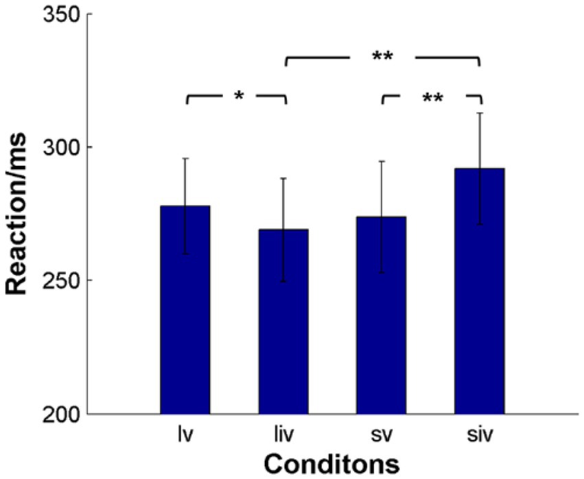
Determine 3. The typical response time (RT) of topics for the 4 circumstances. lv denotes lengthy SOA-valid situation, liv denotes lengthy SOA-invalid situation, sv denotes quick SOA-valid situation, siv denotes quick SOA-valid situation. **p < 0.001, *p < 0.05.

3.2. fMRI outcomes

A single pattern t-test was carried out to research fMRI information, revealing areas associated to visible (V1), auditory (A1), multisensory integration (STG), and a spotlight (angular, center frontal cortex [MFG]) in each the left and proper visible discipline (LVF and RVF). Within the LVF, the principle activated areas (p < 0.05, FDR correction) included the proper angular gyrus (BA39), which is a part of the proper temporoparietal junction (rTPJ), proper STG (BA21), proper Heschl’s gyrus as A1 (BA48), proper lingual gyrus as rV1 (BA18), and proper MFG (BA46), as proven in Determine 4A. Within the RVF, extra activated areas (p < 0.05, FDR correction) included left STG (BA21), left A1 (BA48), left V1 (BA17), bilateral MFG (BAs44/45/46), proper TPJ (BA39), and so forth, as proven in Determine 4B.

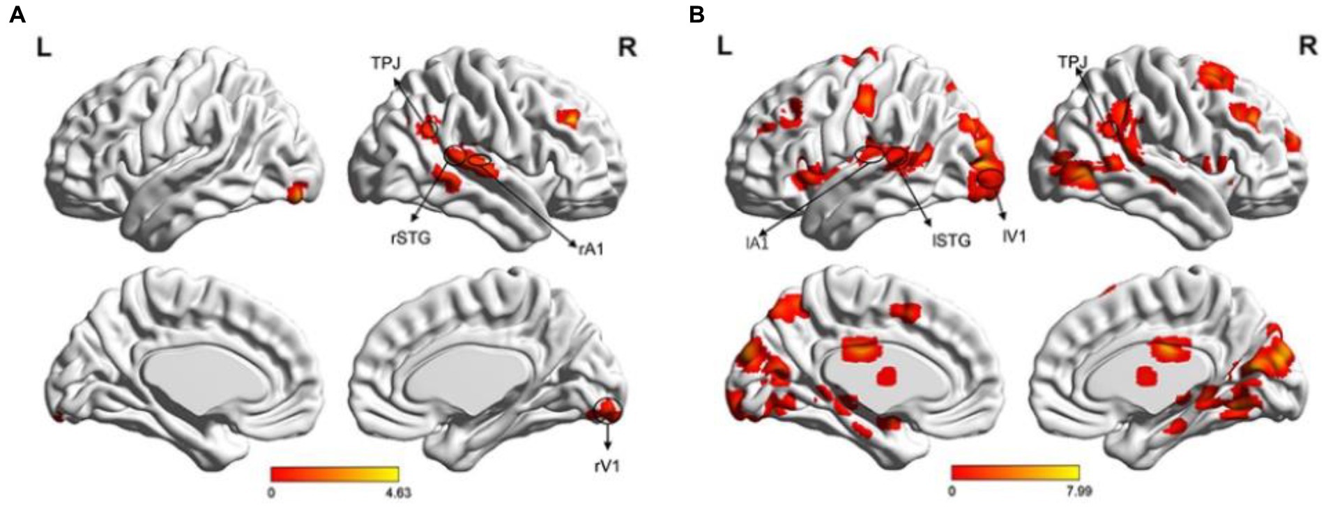
Determine 4. Mind activation maps. (A) Illustration of the activation map when the cue stimulus appeared within the LVF. The primary activated areas (p < 0.05, FDR) included the proper TPJ, proper STG, proper A1, proper V1, and proper MFG; (B) Illustration of the activation map when the cue stimulus appeared within the RVF (p < 0.05, FDR correction). The activated areas included the left STG, left A1, left V1, bilateral MFG, proper TPJ, and proper MT.

We chosen 4 ROIs primarily based on the task-related fMRI activations depicted in Determine 4 for each LVF and RVF cues. Particularly, when the cue appeared in both the LVF or RVF, the proper TPJ (rTPJ) was chosen for each LVF and RVF cues. When the cue appeared within the LVF, we selected the proper STG (rSTG), proper A1 (rA1), and proper V1 (rV1). When the cue appeared within the RVF, we selected the contralateral STG, A1, and V1. The coordinates and sizes of the ROIs are introduced in Desk 1.

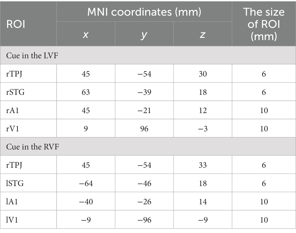
Desk 1. The 4 chosen areas of curiosity (ROIs) in every visible discipline.

3.3. Time-varying community

We computed the time-varying community at time factors starting from 200 ms to 900 ms and displayed the connection time factors solely when it modified within the 4 circumstances. When the cue appeared within the LVF or RVF, the adjustments in cue circumstances have been illustrated in Determine 5A and Determine 5B, respectively. Determine 5C summarizes the outcomes of the time-varying community evaluation. Step one for the lengthy SOA situation was A1↔STG, whereas for the quick SOA situation, it was V1↔STG. The final step for each lengthy and quick SOA circumstances was V1↔STG and STG↔TPJ. Notably, within the lengthy SOA-valid situation, V1↔STG was the center step.

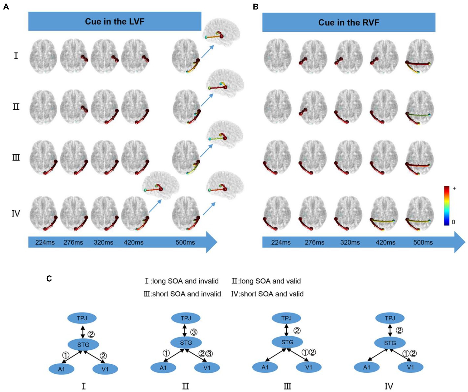
Determine 5. The time-varying networks when the cue stimulus appeared within the (A) LVF and (B) RVF. (C) Abstract of time-varying networks. ①②③ denote the order by which the connections seem.

3.4. Correlation evaluation

Our evaluation revealed important correlations between response and data move (equivalent to STG → TPJ and TPJ → STG) for all circumstances, as proven in Determine 6. For the lengthy SOA, distinct variations have been noticed for every situation. Detrimental correlations have been evident when the cue was invalid and appeared within the LVF (STG → TPJ: r = −0.54, p < 0.05; TPJ → STG: r = −0.52, p < 0.05) or RVF (STG → TPJ: r = −0.51, p < 0.05; TPJ → STG: r = −0.58, p < 0.05). Conversely, optimistic correlations have been evident when the cue was legitimate and appeared in both the LVF (STG → TPJ:r = 0.65, p < 0.01; TPJ → STG: r = 0.52, p < 0.05) or RVF (STG → TPJ:r = 0.53, p < 0.05; TPJ → STG: r = 0.57, p < 0.05). Related developments have been famous for all circumstances for the quick SOA, as proven in Determine 6. Constructive correlations between imply RT and data move have been noticed when the cue was invalid and appeared within the LVF (STG → TPJ: r = 0.59, p < 0.05; TPJ → STG: r = 0.56, p < 0.05) or RVF (STG → TPJ: r = 0.59, p < 0.05; TPJ → STG: r = 0.56, p < 0.05). Equally, optimistic correlations have been noticed when the cue was legitimate, no matter whether or not it appeared within the LVF (STG → TPJ:r = 0.72, p < 0.005 TPJ → STG: r = 0.55, p < 0.05) or RVF (STG → TPJ: r = 0.52, p < 0.05; TPJ → STG: r = 0.53, p < 0.05)

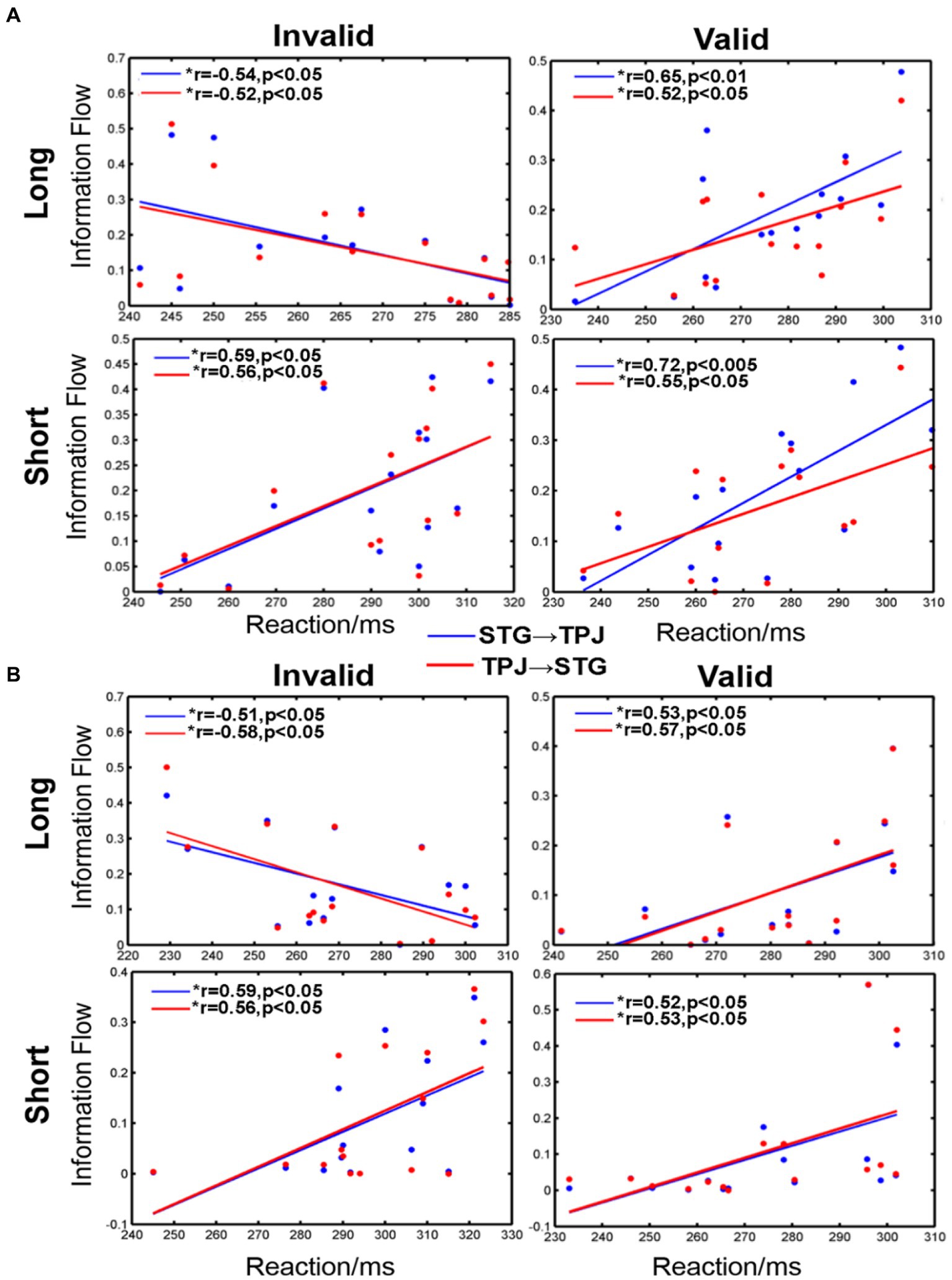
Determine 6. The correlation between data move and common response time (RT) when the cue stimulus appeared within the (A) LVF and (B) RVF. *a major distinction between the 2 areas. STG → TPJ denotes the causal move from STG to TPJ. TPJ → STG denotes the causal move from TPJ to STG.

On this examine, the behavioral outcomes confirmed that the RT for a sound cue was considerably shorter than an invalid cue within the quick SOA situation, whereas the other was reverse for the lengthy SOA, which was just like the unimodal job. In each lengthy and quick SOA circumstances, we noticed STG activation, a important auditory–visible integration area (Klemen and Chambers, 2012). Moreover, we noticed activation in TPJ and MFG, that are vital VAN areas (Corbetta et al., 2008), indicating that spotlight performs a job in auditory–visible integration. Our time-varying community evaluation revealed that V1/A1↔STG occurred earlier than TPJ↔STG, as proven in Determine 5, indicating that pre-attention in auditory–visible integration.

4.1. Related outcomes noticed between the bimodal and unimodal cue-target paradigms

Earlier researches have reported that there’s a important cue impact for brief SOAs within the visible cue-target paradigm. On the situation of the time interval of the cue and goal stimulus is shorter than 300 ms, the topics exhibited quicker responses when the cue was legitimate as in comparison with when it was invalid. Nonetheless, the topics confirmed slower responses when the cue was legitimate slightly than invalid for lengthy SOA (greater than 300 ms). These findings have been per earlier research (Lepsien and Pollmann, 2002; Mayer et al., 2004a,b; Tian and Yao, 2008; Tian et al., 2011) and advised that stimulus-driven consideration results are quicker and extra transient than goal-directed consideration results (Jonides and Irwin, 1981; Shepherd and Müller, 1989; Corbetta et al., 2002; Busse et al., 2008; Macaluso et al., 2016; Tang et al., 2016). Related outcomes have been noticed within the auditory paradigm (Alho et al., 2015; Hanlon et al., 2017). Our behavioral evaluation aligns with earlier analysis on the unimodal paradigm and means that there isn’t any distinction between unimodal and bimodal paradigms within the cue-target paradigm.

4.2. Integration and a spotlight exist within the bimodal cue-target paradigm

Earlier research have emphasised that auditory–visible integration within the cue-target paradigm happens when the cue with one modal stimulus and the goal with a special modal stimulus are introduced from across the similar spatial place (Stein and Meredith, 1990; Spence, 2013; Wu et al., 2020) and at roughly the identical time (Stein and Meredith, 1990; Frassinetti et al., 2002; Bolognini et al., 2005; Spence and Santangelo, 2010; Stevenson et al., 2012; Tang et al., 2016). Nonetheless, it won’t seem if the cue precedes the goal by greater than 300 ms (Spence, 2010). In our paradigm, the time intervals between cue and goal stimulus have been divided into 100 and 800 ms, which can’t be instantly in comparison with earlier research. Our fMRI outcomes, the place the STG appeared in all circumstances, point out that auditory and visible integration happens even when these two stimuli are usually not aligned in area or time (i.e., greater than 300 ms interval).

The position of consideration in multisensory integration remains to be underneath debate. Some research proposed that multisensory integration is an computerized course of (Vroomen et al., 2001; José et al., 2020), whereas others advised that spotlight performed an vital position in multisensory integration (Talsma et al., 2007, 2010; Fairhall and Macaluso, 2009; Tang et al., 2016). Since rTPJ and MFG vital components of the ventral consideration community (Corbetta et al., 2008; Klein et al., 2021), the experimental activation of those rTPJ and MFG advised that spotlight may additionally be concerned in integration. We used time-varying networks to find out the temporal order between multisensory integration and a spotlight utilizing mixture of fMRI and EEG information, which allowed for larger precision than EEG information alone. Moreover, the fMRI information offered a extra exact spatial decision for the time-varying networks.

4.3. Auditory–visible integration previous to consideration

On this analysis, we constructed a time-varying community utilizing task-related fMRI activations as nodes, together with TPJ because the core of the VAN (Corbetta et al., 2008), and STG as an vital space for integration (Yan et al., 2015). Our purpose was to research the connection between multisensory integration and a spotlight. As depicted in Determine 5C, the V1/A1↔STG connection was all the time the primary order, adopted by STG↔TPJ, whatever the circumstances. This discovering helps the notion that pre-attention is concerned in auditory and visible integration, which is per earlier research (Erik et al., 2008). Nonetheless, we noticed some variations underneath totally different circumstances, such because the SOA size. For brief SOA, the primary connection was V1↔STG, as visible stimuli are dominant in processing spatial traits, whereas auditory occasions dominate temporal attribute processing (Bertelson et al., 2000; Stekelenburg et al., 2004; Bonath et al., 2007; Navarra et al., 2010). Conversely, for lengthy SOA, data flowed from the A1 to STG. This outcome is perhaps as a result of auditory–visible stimuli being temporally unsynchronized in our information assortment. Because the SOA elevated, the dominant position of the visible stimulus diminished, and the auditory impact turned stronger, resulting in a major A1↔STG move. Curiously, TPJ↔STG and STG↔V1 have been the final step in all circumstances, indicating that the TPJ modulates the first cortex by utilizing integration areas as a switch node in all instances.

4.4. Relationship between data move and RT

Quite a few research have investigated how consideration impacts a topic’s response time, however there may be disagreement on whether or not consideration boosts or limits the reflection (Senkowski et al., 2005; Karns and Knight, 2009; Macaluso et al., 2016). Some research have advised that spotlight accelerates response velocity (Mcdonald et al., 2005, 2009; Van der Stoep et al., 2017), whereas others have proposed that spotlight may very well inhibit response (Tian and Yao, 2008). A latest examine has demonstrated that each stimulus-driven consideration and multisensory integration can speed up responses (Van der Stoep et al., 2017; Motomura and Amimoto, 2022).

On this examine, we in contrast the correlation between imply RT and the knowledge move of STG↔TPJ underneath totally different circumstances. Our findings counsel that spotlight has a direct affect on multisensory integration, because the extent of data move displays the mutual affect of the 2 mind areas. Particularly, we noticed a destructive correlation between the 2 areas within the lengthy SOA-invalid situation, indicating that bigger data move led to quicker reflection occasions. We inferred that this phenomenon is because of bottom-up consideration, the place elevated data move results in larger data alternate between the STG and TPJ and, thus, quicker reactions. Nonetheless, in different circumstances, we noticed optimistic correlations, which we attribute to the modulation of consideration. Particularly, larger consideration modulation ends in inhibited reactions.

References

Alho, Okay., Salmi, J., Koistinen, S., Salonen, O., and Rinne, T. (2015). High-down managed and bottom-up triggered orienting of auditory consideration to pitch activate overlapping mind networks. Mind Res. 1626, 136–145. doi: 10.1016/j.brainres.2014.12.050
PubMed Summary | CrossRef Full Textual content | Google Scholar
Baenninger, A., Diaz Hernandez, L., Rieger, Okay., Ford, J. M., Kottlow, M., and Koenig, T. (2016). Inefficient preparatory fMRI-BOLD community activations predict working reminiscence dysfunctions in sufferers with schizophrenia. Entrance. Psych. 7:29. doi: 10.3389/fpsyt.2016.00029
Bagshaw, A. P., Hale, J. R., Campos, B. M., Rollings, D. T., Wilson, R. S., Alvim, M. Okay. M., et al. (2017). Sleep onset uncovers thalamic abnormalities in sufferers with idiopathic generalised epilepsy. Neuroimage Clin. 16, 52–57. doi: 10.1016/j.nicl.2017.07.008
Bertelson, P. (1999). Ventriloquism: a case of crossmodal perceptual grouping. Adv. Psychol. 129, 347–362. doi: 10.1016/S0166-4115(99)80034-X
Bertelson, P., Vroomen, J., De, G. B., and Driver, J. (2000). The ventriloquist impact doesn’t rely upon the route of deliberate visible consideration. Percept. Psychophys. 62, 321–332. doi: 10.3758/BF03205552
Bolognini, N., Frassinetti, F., Serino, A., and Làdavas, E. (2005). “Acoustical imaginative and prescient” of beneath threshold stimuli: interplay amongst spatially converging audiovisual inputs. Exp. Mind Res. 160, 273–282. doi: 10.1007/s00221-004-2005-z
Bonath, B., Noesselt, T., Martinez, A., Mishra, J., Schwiecker, Okay., Heinze, H. J., et al. (2007). Neural foundation of the ventriloquist phantasm. Curr. Biol. 17, 1697–1703. doi: 10.1016/j.cub.2007.08.050
Bonte, M., Hausfeld, L., Scharke, W., Valente, G., and Formisano, E. (2014). Process-dependent decoding of speaker and vowel identification from auditory cortical response patterns. J. Neurosci. 34, 4548–4557. doi: 10.1523/JNEUROSCI.4339-13.2014
Branden, J. B., Arvid, G., Mark, P., and Andrew, I. W. (2022). Michael SAG proper temporoparietal junction encodes inferred visible data of others. Neuropsychologia 171:108243. doi: 10.1016/j.neuropsychologia.2022.108243
Bullock, M., Jackson, G. D., and Abbott, D. F. (2021). Artifact discount in simultaneous EEG-fMRI: a scientific evaluate of strategies and modern utilization. Entrance. Neurol. 12:622719. doi: 10.3389/fneur.2021.622719
Busse, L., Katzner, S., and Treue, S. (2008). Temporal dynamics of neuronal modulation throughout exogenous and endogenous shifts of visible consideration in macaque space MT. Proc. Natl. Acad. Sci. 105, 16380–16385. doi: 10.1073/pnas.0707369105
Calvert, G. A., Campbell, R., and Brammer, M. J. (2000). Proof from purposeful magnetic resonance imaging of crossmodal binding within the human heteromodal cortex. Curr. Biol. 10, 649–657. doi: 10.1016/s0960-9822(00)00513-3
Calvert, G. A., Hansen, P. C., Iversen, S. D., and Brammer, M. J. (2001). Detection of audio-visual integration websites in people by utility of electrophysiological standards to the BOLD impact. NeuroImage 14, 427–438. doi: 10.1006/nimg.2001.0812
Calvert, G. A., and Thesen, T. (2004). Multisensory integration: methodological approaches and rising ideas within the human mind. J. Physiol. Paris 98, 191–205. doi: 10.1016/j.jphysparis.2004.03.018
Cappe, C., Thut, G., Romei, V., and Murray, M. M. (2010). Auditory-visual multisensory interactions in people: timing, topography, directionality, and sources. J. Neurosci. 30, 12572–12580. doi: 10.1523/JNEUROSCI.1099-10.2010
Chen, T., Michels, L., Supekar, Okay., Kochalka, J., Ryali, S., and Menon, V. (2015). Position of the anterior insular cortex in integrative causal signaling throughout multisensory auditory-visual consideration. Eur. J. Neurosci. 41, 264–274. doi: 10.1111/ejn.12764
Corbetta, M., Kincade, J. M., and Shulman, G. L. (2002). Neural programs for visible orienting and their relationships to spatial working reminiscence. J. Cogn. Neurosci. 14, 508–523. doi: 10.1162/089892902317362029
Corbetta, M., Patel, G., and Shulman, G. L. (2008). The reorienting system of the human mind: from surroundings to principle of thoughts. Neuron 58, 306–324. doi: 10.1016/j.neuron.2008.04.017
Durk, T., and Woldorff, M. G. (2005). Selective consideration and multisensory integration: a number of phases of results on the evoked mind exercise. J. Cogn. Neurosci. 17, 1098–1114. doi: 10.1162/0898929054475172
Erik, V. D. B., Olivers, C. N. L., Bronkhorst, A. W., and Theeuwes, J. (2008). Pip and pop: nonspatial auditory alerts enhance spatial visible search. J. Exp. Psychol. Hum. Percept. Carry out. 34, 1053–1065. doi: 10.1037/0096-1523.34.5.1053
Fairhall, S. L., and Macaluso, E. (2009). Spatial consideration can modulate audiovisual integration at a number of cortical and subcortical websites. Eur. J. Neurosci. 29, 1247–1257. doi: 10.1111/j.1460-9568.2009.06688.x
Ford, J. M., Roach, B. J., Palzes, V. A., and Mathalon, D. H. (2016). Utilizing concurrent EEG and fMRI to probe the state of the mind in schizophrenia. NeuroImage Clin. 12, 429–441. doi: 10.1016/j.nicl.2016.08.009
Frassinetti, F., Bolognini, N., and Làdavas, E. (2002). Enhancement of visible notion by crossmodal visuo-auditory interplay. Exp. Mind Res. 147, 332–343. doi: 10.1007/s00221-002-1262-y
Friston, Okay. J., Holmes, A. P., Poline, J. B., Grasby, P. J., Williams, S. C. R., Frackowiak, R. S. J., et al. (1995). Evaluation of fMRI time-series revisited. NeuroImage 2, 45–53. doi: 10.1006/nimg.1995.1007
Hanlon, F. M., Dodd, A. B., Ling, J. M., Bustillo, J. R., Abbott, C. C., and Mayer, A. R. (2017). From behavioral facilitation to inhibition: the neuronal correlates of the orienting and reorienting of auditory consideration. Entrance. Hum. Neurosci. 11:293. doi: 10.3389/fnhum.2017.00293
Hsiao, F. C., Tsai, P. J., Wu, C. W., Yang, C. M., Lane, T. J., Lee, H. C., et al. (2018). The neurophysiological foundation of the discrepancy between goal and subjective sleep through the sleep onset interval: an EEG-fMRI examine. Sleep 41:zsy056. doi: 10.1093/sleep/zsy056
José, P., Ossandón, Okay. P., and Heed, T. (2020). No proof for a job of spatially modulated alpha-band exercise in tactile remapping and short-latency, overt orienting habits. J. Neurosci. 40, 9088–9102. doi: 10.1523/JNEUROSCI.0581-19.2020
Kang-jia, J., and Xu, W. (2022). Analysis and Prospect of visible event-related potential in traumatic mind harm and visible operate analysis. J. Forensic Med. 40, 9088–9102. doi: 10.1523/JNEUROSCI.0581-19.2020
Karns, C. M., and Knight, R. T. (2009). Intermodal auditory, visible, and tactile consideration modulates early phases of neural processing. J. Cogn. Neurosci. 21, 669–683. doi: 10.1162/jocn.2009.21037
Klein, H. S., Vanneste, S., and Pinkham, A. E. (2021). The restricted impact of neural stimulation on visible consideration and social cognition in people with schizophrenia. Neuropsychologia 157:107880. doi: 10.1016/j.neuropsychologia.2021.107880
Klemen, J., and Chambers, C. D. (2012). Present views and strategies in learning neural mechanisms of multisensory interactions. Neurosci. Biobehav. Rev. 36, 111–133. doi: 10.1016/j.neubiorev.2011.04.015
Koelewijn, T., Bronkhorst, A., and Theeuwes, J. (2010). Consideration and the a number of phases of multisensory integration: a evaluate of audiovisual research. Acta Psychol. 134, 372–384. doi: 10.1016/j.actpsy.2010.03.010
Laura, B., Roberts, Okay. C., Crist, R. E., Weissman, D. H., and Woldorff, M. G. (2005). The unfold of consideration throughout modalities and area in a multisensory object. Proc. Natl. Acad. Sci. 102, 18751–18756. doi: 10.1073/pnas.0507704102
Li, F., Chen, B., Li, H., Zhang, T., Wang, F., Jiang, Y., et al. (2016). The time-varying networks in P300: a task-evoked EEG examine. IEEE Trans. Neural Syst. Rehabil. Eng. 24, 725–733. doi: 10.1109/TNSRE.2016.2523678
Li, F., Liu, T., Wang, F., Li, H., Gong, D., Zhang, R., et al. (2015). Relationships between the resting-state community and the P3: proof from a scalp EEG examine. Sci. Rep. 5:15129. doi: 10.1038/srep15129
Ľuboš, H., Aaron, R., Seitz,, and Norbert, Okay. (2021). Auditory-visual interactions in selfish distance notion: ventriloquism impact and aftereffecta. J. Acoust. Soc. Am. 150, 3593–3607. doi: 10.1121/10.0007066
Macaluso, E., George, N., Dolan, R., Spence, C., and Driver, J. (2004). Spatial and temporal components throughout processing of audiovisual speech: a PET examine. NeuroImage 21, 725–732. doi: 10.1016/j.neuroimage.2003.09.049
Macaluso, E., Noppeney, U., Talsma, D., Vercillo, T., Hartcher-O’Brien, J., and Adam, R. (2016). The curious incident of consideration in multisensory integration: bottom-up vs High-down. Multisens. Res. 29, 557–583. doi: 10.1163/22134808-00002528
Mastroberardino, S., Santangelo, V., and Macaluso, E. (2015). Crossmodal semantic congruence can have an effect on visuo-spatial processing and exercise of the fronto-parietal consideration networks. Entrance. Integr. Neurosci. 9:45. doi: 10.3389/fnint.2015.00045
Mayer, A. R., Dorflinger, J. M., Rao, S. M., and Seidenberg, M. (2004a). Neural networks underlying endogenous and exogenous visual-spatial orienting. NeuroImage 23, 534–541. doi: 10.1016/j.neuroimage.2004.06.027
Mayer, A., Seidenberg, M., Dorflinger, J., and Rao, S. (2004b). An event-related fMRI examine of exogenous orienting: supporting proof for the cortical foundation of inhibition of return? J. Cogn. Neurosci. 16, 1262–1271. doi: 10.1162/0898929041920531
Mcdonald, J. J., Hickey, C., Inexperienced, J. J., and Whitman, J. C. (2009). Inhibition of return within the covert deployment of consideration: proof from human electrophysiology. J. Cogn. Neurosci. 21, 725–733. doi: 10.1162/jocn.2009.21042
Mcdonald, J. J., Teder-Sälejärvi, W. A., Di, R. F., and Hillyard, S. A. (2005). Neural foundation of auditory-induced shifts in visible time-order notion. Nat. Neurosci. 8, 1197–1202. doi: 10.1038/nn1512
Mesgarani, N., Cheung, C., Johnson, Okay., and Chang, E. F. (2014). Phonetic function encoding in human superior temporal gyrus. Science 343, 1006–1010. doi: 10.1126/science.1245994
Motomura, Okay., and Amimoto, Okay. (2022). Growth of stimulus-driven consideration check for unilateral spatial neglect – accuracy, reliability, and validity. Neurosci. Lett. 772:136461. doi: 10.1016/j.neulet.2022.136461
Muraskin, J., Brown, T. R., Walz, J. M., Tu, T., Conroy, B., Goldman, R. I., et al. (2018). A multimodal encoding mannequin utilized to imaging decision-related neural cascades within the human mind. NeuroImage 180, 211–222. doi: 10.1016/j.neuroimage.2017.06.059
Navarra, J., Soto-Faraco, S., and Spence, C. (2010). Assessing the position of consideration within the audiovisual integration of speech. Inf. Fusion 11, 4–11. doi: 10.1016/j.inffus.2009.04.001
Nazir, H. M., Hussain, I., Faisal, M., Mohamd Shoukry, A., Abdel Wahab Sharkawy, M., Fawzi Al-Deek, F., et al. (2020). Dependence construction evaluation of multisite river influx information utilizing vine copula-CEEMDAN primarily based hybrid mannequin. PeerJ 8:e10285. doi: 10.7717/peerj.10285
Noesselt, T., Rieger, J. W., Schoenfeld, M. A., Kanowski, M., Hinrichs, H., Heinze, H. J., et al. (2007). Audiovisual temporal correspondence modulates human multisensory superior temporal sulcus plus major sensory cortices. J. Neurosci. 27, 11431–11441. doi: 10.1523/JNEUROSCI.2252-07.2007
Pisauro, M. A., Fouragnan, E., Retzler, C., and Philiastides, M. G. (2017). Neural correlates of proof accumulation throughout value-based choices revealed by way of simultaneous EEG-fMRI. Nat. Commun. 8:15808. doi: 10.1038/ncomms15808
Platt, B. B., and Warren, D. H. (1972). Auditory localization: the significance of eye actions and a textured visible surroundings. Percept. Psychophys. 12, 245–248. doi: 10.3758/BF03212884
Posner, M. I., and Rothbart, M. Okay. (2006). Analysis on consideration networks as a mannequin for the combination of psychological science. Annu. Rev. Psychol. 58, 1–23. doi: 10.1146/annurev.psych.58.110405.085516
Rachel, W., Kathleen, B., and Mark, A. (2022). Evaluating the co-design of an age-friendly, rural, multidisciplinary major care mannequin: a examine protocol. Strategies Protoc. 5:23. doi: 10.3390/mps5020023
Romei, V., Murray, M. M., Cappe, C., and Thut, G. (2013). The contributions of sensory dominance and attentional Bias to cross-modal enhancement of visible cortex excitability. J. Cogn. Neurosci. 25, 1122–1135. doi: 10.1162/jocn_a_00367
Rupp, Okay., Hect, J. L., Remick, M., Ghuman, A., Chandrasekaran, B., Holt, L. L., et al. (2022). Neural responses in human superior temporal cortex help coding of voice representations. PLoS Biol. 20:e3001675. doi: 10.1371/journal.pbio.3001675
Sébastien, A. L., Arin, E. A., Kristina, C., Blake, E. B., and Ryan, A. S. (2022). The connection between multisensory associative studying and multisensory integration. Neuropsychologia 174:108336. doi: 10.1016/j.neuropsychologia.2022.108336
Senkowski, D., Talsma, D., Herrmann, C. S., and Woldorff, M. G. (2005). Multisensory processing and oscillatory gamma responses: results of spatial selective consideration. Exp. Mind Res. 166, 411–426. doi: 10.1007/s00221-005-2381-z
Shams, L., Kamitani, Y., and Shimojo, S. (2000). What you see is what you hear. Nature 408, 788–2671. doi: 10.1038/35048669
Shams, N., Alain, C., and Strother, S. (2015). Comparability of BCG artifact elimination strategies for evoked responses in simultaneous EEG-fMRI. J. Neurosci. Strategies 245, 137–146. doi: 10.1016/j.jneumeth.2015.02.018
Shepherd, M., and Müller, H. J. (1989). Motion versus focusing of visible consideration. Percept. Psychophys. 46, 146–154. doi: 10.3758/BF03204974
Spence, C. (2010). Crossmodal spatial consideration. Ann. N. Y. Acad. Sci. 1191, 182–200. doi: 10.1111/j.1749-6632.2010.05440.x
Spence, C., and Santangelo, V. (2010). Auditory growth and studying. Oxf. Handb. Audit. Sci. 3:249. doi: 10.1093/oxfordhb/9780199233557.013.0013
Stein, B. E., and Meredith, M. A. (1990). Multisensory integration. Neural and behavioral options for coping with stimuli from totally different sensory modalities. Ann. N. Y. Acad. Sci. 608, 51–70. doi: 10.1111/j.1749-6632.1990.tb48891.x
Stein, B. E., Meredith, M. A., Huneycutt, W. S., and Mcdade, L. (1989). Behavioral indices of multisensory integration: orientation to visible cues is affected by auditory stimuli. J. Cogn. Neurosci. 1, 12–24. doi: 10.1162/jocn.1989.1.1.12
Stekelenburg, J. J., Vroomen, J., and De, G. B. (2004). Illusory sound shifts induced by the ventriloquist phantasm evoke the mismatch negativity. Neurosci. Lett. 357, 163–166. doi: 10.1016/j.neulet.2003.12.085
Stevenson, R. A., Fister, J. Okay., Barnett, Z. P., Nidiffer, A. R., and Wallace, M. T. (2012). Interactions between the spatial and temporal stimulus components that affect multisensory integration in human efficiency. Exp. Mind Res. 219, 121–137. doi: 10.1007/s00221-012-3072-1
Stoep, N., Der, V., Stigchel, S., Der, V., and Nijboer, T. C. W. (2015). Exogenous spatial consideration decreases audiovisual integration. Atten. Percept. Psychophys. 77, 464–482. doi: 10.3758/s13414-014-0785-1
Talsma, D., Doty, T. J., and Woldorff, M. G. (2007). Selective consideration and audivisual integration: is attending to each modalities a prerequisite for optimum early integration? Cereb. Cortex 17, 691–701. doi: 10.1093/cercor/bhk020
Talsma, D., Senkowski, D. F. S., and Woldorff, M. G. (2010). The multifaceted interaction between consideration and multisensory integration. Tendencies Cogn. Sci. 14, 400–410. doi: 10.1016/j.tics.2010.06.008
Tang, X., Wu, J., and Shen, Y. (2016). The interactions of multisensory integration with endogenous andexogenous consideration. Neurosci. Biobehav. Rev. 61, 208–224. doi: 10.1016/j.neubiorev.2015.11.002
Tedersälejärvi, W. A., Di, R. F., Mcdonald, J. J., and Hillyard, S. A. (2005). Results of spatial congruity on audio-visual multimodal integration. J. Cogn. Neurosci. 17, 1396–1409. doi: 10.1162/0898929054985383
Tian, Y., Klein, R. M., Satel, J., Xu, P., and Yao, D. (2011). Electrophysiological explorations of the trigger and impact of inhibition of return in a Cue-target paradigm. Mind Topogr. 24, 164–182. doi: 10.1007/s10548-011-0172-3
Tian, Y., Liang, S., and Yao, D. (2014). Attentional orienting and response inhibition: insights from spatial-temporal neuroimaging. Neurosci. Bull. 30, 141–152. doi: 10.1007/s12264-013-1372-5
Tian, Y., and Ma, L. (2020). Auditory consideration monitoring states in a cocktail celebration surroundings may be decoded by deep convolutional neural networks. J. Neural Eng. 17:036013. doi: 10.1088/1741-2552/ab92b2
Tian, Y., Xu, W., and Yang, L. (2018a). Cortical classification with rhythm entropy for error processing in cocktail celebration surroundings primarily based on scalp EEG recording. Sci. Rep. 8:6070. doi: 10.1038/s41598-018-24535-4
Tian, Y., Xu, W., Zhang, H., Tam, Okay. Y., Zhang, H., Yang, L., et al. (2018b). The scalp time-varying networks of N170: reference, latency, and data move. Entrance. Neurosci. 12:250. doi: 10.3389/fnins.2018.00250
Tian, Y., and Yao, D. (2008). A examine on the neural mechanism of inhibition of return by the event-related potential within the go/Nogo job. Biol. Psychol. 79, 171–178. doi: 10.1016/j.biopsycho.2008.04.006
Tian, Y., and Yao, D. (2013). Why do we have to use a zero reference? Reference influences on the ERPs of audiovisual results. Psychophysiology 50, 1282–1290. doi: 10.1111/psyp.12130
Van der Stoep, N., Van der Stigchel, S., Nijboer, T. C., and Spence, C. (2017). Visually induced inhibition of return impacts the combination of auditory and visible data. Notion 46, 6–17. doi: 10.1177/0301006616661934
Vroomen, J., Bertelson, P., and Gelder, B. D. (2001). Directing spatial consideration in the direction of the illusory location of a ventriloquized sound. Acta Psychol. 108, 21–33. doi: 10.1016/S0001-6918(00)00068-8
Wang, Okay., Li, W., and Dong, L. (2018). Clustering-constrained ICA for Ballistocardiogram artifacts elimination in simultaneous EEG-fMRI. Entrance. Neurosci. 12:59. doi: 10.3389/fnins.2018.00059
Wang, P., Fuentes, L. J., Vivas, A. B., and Chen, Q. (2013). Behavioral and neural interplay between spatial inhibition of return and the Simon impact. Entrance. Hum. Neurosci. 7:572. doi: 10.3389/fnhum.2013.00572
Wang, W., Wang, Y., Solar, J., Liu, Q., Liang, J., and Li, T. (2020). Speech pushed speaking head era by way of attentional landmarks primarily based illustration. Proc. Interspeech 2020, 1326–1330. doi: 10.21437/Interspeech.2020-2304
Wen, H., You, S., and Fu, Y. (2021). Cross-modal dynamic convolution for multi-modal emotion recognition. J. Vis. Commun. Picture Characterize. 78:103178. doi: 10.1016/j.jvcir.2021.103178
Wilke, C., Ding, L., and He, B. (2008). Estimation of time-varying connectivity patterns by the usage of an adaptive directed switch operate. IEEE Trans. Biomed. Eng. 55, 2557–2564. doi: 10.1109/TBME.2008.919885
Xu, Z., Yang, W., and Zhou, Z. (2020). Cue–goal onset asynchrony modulates interplay between exogenous consideration and audiovisual integration. Cogn. Course of. 21, 261–270. doi: 10.1007/s10339-020-00950-2
Yan, T., Geng, Y., Wu, J., and Li, C. (2015). Interactions between multisensory inputs with voluntary spatial consideration: an fMRI examine. Neuroreport 26, 605–612. doi: 10.1097/WNR.0000000000000368
Yao, D., Li, W., Oostenveld, R., Nielsen, Okay. D., Arendt-Nielsen, L., and Chen, C. A. N. (2005). A comparative examine of various references for EEG spectral mapping: the difficulty of the impartial reference and the usage of the infinity reference. Physiol. Meas. 26, 173–184. doi: 10.1088/0967-3334/26/3/003
Zhang, J., Li, Y., Li, T., Xun, L., and Shan, C. (2019). License plate localization in unconstrained scenes utilizing a two-stage CNN-RNN. IEEE Sensors J. 19, 5256–5265. doi: 10.1109/JSEN.2019.2900257
Zhang, T., Gao, Y., and Hu, S. (2022). Targeted consideration: its key position in gaze and arrow cues for figuring out the place consideration is directed. Psychol. Res. 2022, 1–15. doi: 10.1007/s00426-022-01781-w
Zhang, X., Wang, Z., and Liu, T. (2022). Anti-disturbance built-in place synchronous management of a twin everlasting magnet synchronous motor system. Energies 15:6697. doi: 10.3390/en15186697